Understanding random variables and probability helps us make sense of...
Understanding Discrete and Continuous Random Variables: Probability Distributions Made Easy


1 / 10
1
of 10
Understanding Discrete and Continuous Random Variables
Random variables are fundamental concepts in probability theory that help us quantify outcomes of chance events. Discrete and continuous random variables represent two distinct ways that random phenomena can be measured and analyzed.
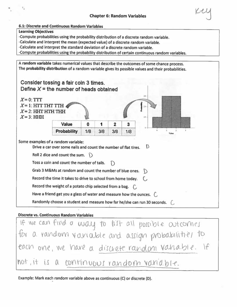
A discrete random variable takes on specific, countable values with gaps between them. For example, when counting the number of heads in three coin tosses, the possible values are 0, 1, 2, or 3 - nothing in between. Each outcome has a specific probability, creating what we call a probability distribution.
Definition: A discrete random variable has countable, separate values while a continuous random variable can take any value within a range.
In contrast, continuous random variables can take any value within a range. Think about measuring time, distance, or weight - these can be any number within their possible ranges. For instance, a student's running time for 30 seconds could be 27.32 seconds, 27.325 seconds, or any other precise measurement.
Example: When rolling two dice and summing their values, you have a discrete random variable . When measuring the time to drive to school, you have a continuous random variable (any positive number of minutes).
The key distinction lies in whether you can list all possible outcomes. If you can enumerate every possible value and assign specific probabilities to each, it's discrete. If the values flow continuously with infinitely many possibilities between any two values, it's continuous.
2
of 10
Probability Distributions and Their Properties
Understanding probability distributions for random variables is crucial for analyzing chance events. For discrete random variables, the probability distribution provides a complete list of possible values and their corresponding probabilities.
When working with probability distributions, two fundamental rules must always be satisfied:
- Each individual probability must be between 0 and 1
- The sum of all probabilities must equal exactly 1
Highlight: A valid probability distribution must have probabilities that sum to 1, representing all possible outcomes of the random variable.
Creating a histogram of probability distribution for random variables helps visualize the shape and characteristics of the distribution. For example, when analyzing roller coaster inversions, the histogram might show a right-skewed distribution, meaning most roller coasters have few inversions while a small number have many.
The practical application of probability distributions extends to many fields. Insurance companies use them to model claim frequencies, quality control departments use them to track defects, and scientists use them to analyze experimental outcomes.
3
of 10
Calculating Mean and Standard Deviation
Calculating mean and standard deviation of discrete random variables provides crucial information about the center and spread of probability distributions. The mean (expected value) represents the long-term average outcome if the random process were repeated many times.
To calculate the mean of a discrete random variable:
- Multiply each possible value by its probability
- Sum all these products
- The result represents the theoretical average outcome
Example: For a roulette wheel bet on red, if X represents the net gain:
- Winning: +$1 with probability 18/38
- Losing: -$1 with probability 20/38
- Expected value = (1)(18/38) + (-1)(20/38) = -$0.05
The standard deviation measures the typical deviation from the mean, providing insight into the variability of outcomes. It's calculated by:
- Finding the difference between each value and the mean
- Squaring these differences
- Multiplying by their respective probabilities
- Summing these products
- Taking the square root of the result
Vocabulary: The variance is the square of the standard deviation and represents the average squared deviation from the mean.
4
of 10
Applications and Interpretations
Practical applications of random variables and their distributions appear throughout science, business, and everyday life. Understanding these concepts helps in making informed decisions under uncertainty.
When analyzing real-world scenarios, it's important to interpret statistical measures in context. For example, in a car dealership's sales data, the mean represents the average number of cars sold per hour, while the standard deviation indicates how much typical sales vary from this average.
Definition: The expected value (mean) represents the theoretical long-term average outcome, while the standard deviation measures the typical variation from this average.
Statistical software and calculators can help perform these calculations efficiently. When using technology:
- Enter the values of the random variable
- Input corresponding probabilities
- Use built-in functions to calculate summary statistics
Highlight: Always interpret results in the context of the original problem, maintaining units and practical significance of the calculations.
5
of 10
Understanding Continuous Random Variables and Probability Distributions
A discrete and continuous random variables probability distribution represents fundamentally different ways that random events can occur. While discrete variables take specific values, continuous random variables can take any value within a range. The probability distribution for continuous variables is described by a smooth density curve, where the total area under the curve equals 1.
When working with continuous random variables, we focus on intervals rather than specific points. This is because the probability of any exact value is actually zero - we can only measure the probability of values falling within a range. For example, when measuring human height, we might want to know the probability of someone being between 5'8" and 5'10", rather than exactly 5'9".
Definition: A continuous random variable is a variable that can take on any value within a specified interval. The probability of the variable falling within any interval is equal to the area under the density curve above that interval.
The relationship between different probability calculations becomes particularly important. For continuous variables, P(X < a) equals P(X ≤ a) because the probability of hitting exactly point a is zero. This property helps simplify many probability calculations and is crucial for understanding continuous distributions.
6
of 10
Normal Distributions and Their Applications
The Normal distribution is one of the most important continuous probability distributions, often appearing in natural phenomena. When working with Normal distributions, we can calculate probabilities using standardized methods and tables.
Example: Consider heights of two-year-old males following a Normal distribution with mean μ = 34 inches and standard deviation σ = 1.4 inches. To find the probability of a randomly selected child being at least 33 inches tall, we can use standardized Normal calculations or technology tools.
Understanding how to interpret these probabilities in real-world contexts is crucial. For instance, if we calculate that P(32 < X < 36) = 0.8469, this means about 84.69% of two-year-old males have heights between 32 and 36 inches. This type of interpretation makes statistics practical and meaningful.
Highlight: When working with Normal distributions, always remember that approximately 68% of data falls within one standard deviation of the mean, 95% within two standard deviations, and 99.7% within three standard deviations.
7
of 10
Transforming Random Variables and Their Properties
Understanding how mathematical operations affect random variables is essential for statistical analysis. When we transform random variables through addition, subtraction, multiplication, or division, their properties change in predictable ways.
Vocabulary: Linear transformations include adding, subtracting, multiplying, or dividing a random variable by constants. These transformations affect the mean and standard deviation of the distribution in specific ways.
The effects of linear transformations follow clear patterns:
- Adding or subtracting a constant changes the mean but not the spread
- Multiplying or dividing by a constant affects both the mean and standard deviation
- The shape of the distribution remains unchanged for positive multipliers
Definition: For a linear transformation Y = a + bX:
- The mean of Y equals a + bμx
- The standard deviation of Y equals |b|σx
- The shape remains the same if b > 0
8
of 10
Practical Applications of Random Variable Transformations
Real-world applications of random variable transformations appear frequently in business and engineering contexts. Consider a car dealership tracking sales and calculating bonuses based on those sales.
When analyzing financial outcomes, we often need to transform basic count data into monetary values. For example, if X represents the number of items sold and each sale earns $500, the total earnings Y would be 500X. This transformation affects both the mean and standard deviation of the distribution.
Example: If a car dealership's hourly sales follow a distribution with mean 1.1 and standard deviation 0.94, and each sale earns a $500 bonus, the bonus distribution will have:
- Mean = $500(1.1) = $550
- Standard deviation = $500(0.94) = $470
Understanding these transformations helps in making business decisions and predictions about financial outcomes. The ability to calculate and interpret these transformed distributions is crucial for practical applications in business and other fields.
9
of 10
Understanding Combined Random Variables and Their Properties
When working with multiple random variables, understanding how to combine them is crucial for statistical analysis. This exploration focuses on how to handle discrete and continuous random variables when they are added or subtracted, particularly regarding their means and variances.
Definition: Combined random variables occur when we perform mathematical operations (like addition or subtraction) on two or more separate random variables to create a new random variable.
The mean of combined random variables follows straightforward rules. When adding two random variables X and Y to form T = X + Y, the mean of T equals the sum of the individual means . This principle extends to any number of random variables being added together. For example, if you're tracking both daily rainfall (X) and daily temperature (Y), the mean of their sum will equal the sum of their individual means.
Independence between random variables plays a crucial role in probability calculations. Two random variables are considered independent when the occurrence of events related to one variable doesn't affect the probability of events related to the other. This concept is particularly important when calculating mean and standard deviation of discrete random variables.
Highlight: When working with independent random variables, the variance of their sum equals the sum of their individual variances. However, this rule only applies when the variables are truly independent.
10
of 10
Analyzing Differences Between Random Variables and Variance Properties
Understanding how random variables behave when subtracted from each other is essential for statistical analysis, particularly when examining differences between datasets or comparing variables. This knowledge helps in creating accurate probability distributions and analyzing data variations.
When finding the difference between random variables , the mean of the difference equals the difference of their means . The order of subtraction matters significantly - subtracting Y from X produces a different result than subtracting X from Y. This principle is crucial when analyzing comparative data, such as comparing test scores between different groups.
Example: If X represents scores from Group A with a mean of 85, and Y represents scores from Group B with a mean of 75, then D = X - Y would have a mean of 10 points, indicating the average difference between the groups.
The variance of differences between independent random variables follows the same rule as the variance of sums - it equals the sum of individual variances. This might seem counterintuitive, but it's a fundamental principle in probability theory. When working with standard deviations, it's crucial to remember that you cannot simply add or subtract them - you must work with variances first and then take the square root if needed.
Vocabulary: Variance measures the spread of data points around the mean, while standard deviation is the square root of variance, providing a measure of dispersion in the same units as the original data.
We thought you’d never ask...
What is the Knowunity AI companion?
Our AI companion is specifically built for the needs of students. Based on the millions of content pieces we have on the platform we can provide truly meaningful and relevant answers to students. But its not only about answers, the companion is even more about guiding students through their daily learning challenges, with personalised study plans, quizzes or content pieces in the chat and 100% personalisation based on the students skills and developments.
Where can I download the Knowunity app?
You can download the app in the Google Play Store and in the Apple App Store.
Is Knowunity really free of charge?
That's right! Enjoy free access to study content, connect with fellow students, and get instant help – all at your fingertips.
Most popular content in AP Statistics
2I
Introduction to Bivariate Quantitative Data
Students will practice identifying explanatory and response variables and interpreting scatterplots for direction, form, strength, and outliers.
9th3180
Hypothesis Testing Project
statistics project using null and alternative hypotheses and how they can be interpreted
20111
Most popular content
9O
Origins and Dynamics of the Columbian Exchange
Analyze the ecological and economic motivations behind the initial transfer of goods, people, and diseases between the Old and New Worlds.
9th3,1280
I
Introduction to Early Cultural Interactions
Analyze the initial social and religious encounters between Europeans, Africans, and Indigenous peoples in the colonial Americas.
9th2,7730
O
Origins of Ancient River Civilizations
Analyze the environmental factors and technological innovations that led to the rise of early states in Mesopotamia, Egypt, and the Indus Valley.
9th3,1870
M
Motivations for European Exploration
Analyze the economic, religious, and political factors that drove European powers to the Americas during the 15th and 16th centuries.
9th1,7780
F
Foundations of Ethical Guidelines in Research
Practice the core principles of the APA ethical code including informed consent, debriefing, and the role of Institutional Review Boards.
9th1,3360
I
Introduction to Native American Societies
Examine the diverse social, political, and economic structures of North American indigenous groups prior to European contact.
9th1,1100
I
Introduction to Biological Elements of Life
Practice identifying the essential elements including carbon, nitrogen, phosphorus, and sulfur that compose biological macromolecules.
9th1,7390
I
Introduction to the Spanish Encomienda System
Explore the fundamental economic and social structures of the Spanish colonial system, focusing on the encomienda and the casta social hierarchy.
9th8890
O
Origins and Continuity of the Byzantine Empire
Analyze the political and cultural transitions from the Roman Empire to the Byzantine Empire, focusing on the reign of Justinian I and his code.
9th1,6320
Can't find what you're looking for? Explore other subjects.
Students love us — and so will you.
4.6/5App Store
4.7/5Google Play
The app is very easy to use and well designed. I have found everything I was looking for so far and have been able to learn a lot from the presentations! I will definitely use the app for a class assignment! And of course it also helps a lot as an inspiration.
Stefan SiOS user
This app is really great. There are so many study notes and help [...]. My problem subject is French, for example, and the app has so many options for help. Thanks to this app, I have improved my French. I would recommend it to anyone.
Samantha KlichAndroid user
Wow, I am really amazed. I just tried the app because I've seen it advertised many times and was absolutely stunned. This app is THE HELP you want for school and above all, it offers so many things, such as workouts and fact sheets, which have been VERY helpful to me personally.
AnnaiOS user
Understanding Discrete and Continuous Random Variables: Probability Distributions Made Easy
Understanding random variables and probability helps us make sense of uncertain events in the real world.
Discrete and continuous random variablesare fundamental concepts in probability theory. A discrete random variable can only take specific, separate values (like the number...
1
of 10
Sign up to see the content. It's free!
- Access to all documents
- Improve your grades
- Join milions of students
Understanding Discrete and Continuous Random Variables
Random variables are fundamental concepts in probability theory that help us quantify outcomes of chance events. Discrete and continuous random variables represent two distinct ways that random phenomena can be measured and analyzed.
A discrete random variable takes on specific, countable values with gaps between them. For example, when counting the number of heads in three coin tosses, the possible values are 0, 1, 2, or 3 - nothing in between. Each outcome has a specific probability, creating what we call a probability distribution.
Definition: A discrete random variable has countable, separate values while a continuous random variable can take any value within a range.
In contrast, continuous random variables can take any value within a range. Think about measuring time, distance, or weight - these can be any number within their possible ranges. For instance, a student's running time for 30 seconds could be 27.32 seconds, 27.325 seconds, or any other precise measurement.
Example: When rolling two dice and summing their values, you have a discrete random variable . When measuring the time to drive to school, you have a continuous random variable (any positive number of minutes).
The key distinction lies in whether you can list all possible outcomes. If you can enumerate every possible value and assign specific probabilities to each, it's discrete. If the values flow continuously with infinitely many possibilities between any two values, it's continuous.
2
of 10Sign up to see the content. It's free!
- Access to all documents
- Improve your grades
- Join milions of students
Probability Distributions and Their Properties
Understanding probability distributions for random variables is crucial for analyzing chance events. For discrete random variables, the probability distribution provides a complete list of possible values and their corresponding probabilities.
When working with probability distributions, two fundamental rules must always be satisfied:
- Each individual probability must be between 0 and 1
- The sum of all probabilities must equal exactly 1
Highlight: A valid probability distribution must have probabilities that sum to 1, representing all possible outcomes of the random variable.
Creating a histogram of probability distribution for random variables helps visualize the shape and characteristics of the distribution. For example, when analyzing roller coaster inversions, the histogram might show a right-skewed distribution, meaning most roller coasters have few inversions while a small number have many.
The practical application of probability distributions extends to many fields. Insurance companies use them to model claim frequencies, quality control departments use them to track defects, and scientists use them to analyze experimental outcomes.
3
of 10Sign up to see the content. It's free!
- Access to all documents
- Improve your grades
- Join milions of students
Calculating Mean and Standard Deviation
Calculating mean and standard deviation of discrete random variables provides crucial information about the center and spread of probability distributions. The mean (expected value) represents the long-term average outcome if the random process were repeated many times.
To calculate the mean of a discrete random variable:
- Multiply each possible value by its probability
- Sum all these products
- The result represents the theoretical average outcome
Example: For a roulette wheel bet on red, if X represents the net gain:
- Winning: +$1 with probability 18/38
- Losing: -$1 with probability 20/38
- Expected value = (1)(18/38) + (-1)(20/38) = -$0.05
The standard deviation measures the typical deviation from the mean, providing insight into the variability of outcomes. It's calculated by:
- Finding the difference between each value and the mean
- Squaring these differences
- Multiplying by their respective probabilities
- Summing these products
- Taking the square root of the result
Vocabulary: The variance is the square of the standard deviation and represents the average squared deviation from the mean.
4
of 10Sign up to see the content. It's free!
- Access to all documents
- Improve your grades
- Join milions of students
Applications and Interpretations
Practical applications of random variables and their distributions appear throughout science, business, and everyday life. Understanding these concepts helps in making informed decisions under uncertainty.
When analyzing real-world scenarios, it's important to interpret statistical measures in context. For example, in a car dealership's sales data, the mean represents the average number of cars sold per hour, while the standard deviation indicates how much typical sales vary from this average.
Definition: The expected value (mean) represents the theoretical long-term average outcome, while the standard deviation measures the typical variation from this average.
Statistical software and calculators can help perform these calculations efficiently. When using technology:
- Enter the values of the random variable
- Input corresponding probabilities
- Use built-in functions to calculate summary statistics
Highlight: Always interpret results in the context of the original problem, maintaining units and practical significance of the calculations.
5
of 10Sign up to see the content. It's free!
- Access to all documents
- Improve your grades
- Join milions of students
Understanding Continuous Random Variables and Probability Distributions
A discrete and continuous random variables probability distribution represents fundamentally different ways that random events can occur. While discrete variables take specific values, continuous random variables can take any value within a range. The probability distribution for continuous variables is described by a smooth density curve, where the total area under the curve equals 1.
When working with continuous random variables, we focus on intervals rather than specific points. This is because the probability of any exact value is actually zero - we can only measure the probability of values falling within a range. For example, when measuring human height, we might want to know the probability of someone being between 5'8" and 5'10", rather than exactly 5'9".
Definition: A continuous random variable is a variable that can take on any value within a specified interval. The probability of the variable falling within any interval is equal to the area under the density curve above that interval.
The relationship between different probability calculations becomes particularly important. For continuous variables, P(X < a) equals P(X ≤ a) because the probability of hitting exactly point a is zero. This property helps simplify many probability calculations and is crucial for understanding continuous distributions.
6
of 10Sign up to see the content. It's free!
- Access to all documents
- Improve your grades
- Join milions of students
Normal Distributions and Their Applications
The Normal distribution is one of the most important continuous probability distributions, often appearing in natural phenomena. When working with Normal distributions, we can calculate probabilities using standardized methods and tables.
Example: Consider heights of two-year-old males following a Normal distribution with mean μ = 34 inches and standard deviation σ = 1.4 inches. To find the probability of a randomly selected child being at least 33 inches tall, we can use standardized Normal calculations or technology tools.
Understanding how to interpret these probabilities in real-world contexts is crucial. For instance, if we calculate that P(32 < X < 36) = 0.8469, this means about 84.69% of two-year-old males have heights between 32 and 36 inches. This type of interpretation makes statistics practical and meaningful.
Highlight: When working with Normal distributions, always remember that approximately 68% of data falls within one standard deviation of the mean, 95% within two standard deviations, and 99.7% within three standard deviations.
7
of 10Sign up to see the content. It's free!
- Access to all documents
- Improve your grades
- Join milions of students
Transforming Random Variables and Their Properties
Understanding how mathematical operations affect random variables is essential for statistical analysis. When we transform random variables through addition, subtraction, multiplication, or division, their properties change in predictable ways.
Vocabulary: Linear transformations include adding, subtracting, multiplying, or dividing a random variable by constants. These transformations affect the mean and standard deviation of the distribution in specific ways.
The effects of linear transformations follow clear patterns:
- Adding or subtracting a constant changes the mean but not the spread
- Multiplying or dividing by a constant affects both the mean and standard deviation
- The shape of the distribution remains unchanged for positive multipliers
Definition: For a linear transformation Y = a + bX:
- The mean of Y equals a + bμx
- The standard deviation of Y equals |b|σx
- The shape remains the same if b > 0
8
of 10Sign up to see the content. It's free!
- Access to all documents
- Improve your grades
- Join milions of students
Practical Applications of Random Variable Transformations
Real-world applications of random variable transformations appear frequently in business and engineering contexts. Consider a car dealership tracking sales and calculating bonuses based on those sales.
When analyzing financial outcomes, we often need to transform basic count data into monetary values. For example, if X represents the number of items sold and each sale earns $500, the total earnings Y would be 500X. This transformation affects both the mean and standard deviation of the distribution.
Example: If a car dealership's hourly sales follow a distribution with mean 1.1 and standard deviation 0.94, and each sale earns a $500 bonus, the bonus distribution will have:
- Mean = $500(1.1) = $550
- Standard deviation = $500(0.94) = $470
Understanding these transformations helps in making business decisions and predictions about financial outcomes. The ability to calculate and interpret these transformed distributions is crucial for practical applications in business and other fields.
9
of 10Sign up to see the content. It's free!
- Access to all documents
- Improve your grades
- Join milions of students
Understanding Combined Random Variables and Their Properties
When working with multiple random variables, understanding how to combine them is crucial for statistical analysis. This exploration focuses on how to handle discrete and continuous random variables when they are added or subtracted, particularly regarding their means and variances.
Definition: Combined random variables occur when we perform mathematical operations (like addition or subtraction) on two or more separate random variables to create a new random variable.
The mean of combined random variables follows straightforward rules. When adding two random variables X and Y to form T = X + Y, the mean of T equals the sum of the individual means . This principle extends to any number of random variables being added together. For example, if you're tracking both daily rainfall (X) and daily temperature (Y), the mean of their sum will equal the sum of their individual means.
Independence between random variables plays a crucial role in probability calculations. Two random variables are considered independent when the occurrence of events related to one variable doesn't affect the probability of events related to the other. This concept is particularly important when calculating mean and standard deviation of discrete random variables.
Highlight: When working with independent random variables, the variance of their sum equals the sum of their individual variances. However, this rule only applies when the variables are truly independent.
10
of 10Sign up to see the content. It's free!
- Access to all documents
- Improve your grades
- Join milions of students
Analyzing Differences Between Random Variables and Variance Properties
Understanding how random variables behave when subtracted from each other is essential for statistical analysis, particularly when examining differences between datasets or comparing variables. This knowledge helps in creating accurate probability distributions and analyzing data variations.
When finding the difference between random variables , the mean of the difference equals the difference of their means . The order of subtraction matters significantly - subtracting Y from X produces a different result than subtracting X from Y. This principle is crucial when analyzing comparative data, such as comparing test scores between different groups.
Example: If X represents scores from Group A with a mean of 85, and Y represents scores from Group B with a mean of 75, then D = X - Y would have a mean of 10 points, indicating the average difference between the groups.
The variance of differences between independent random variables follows the same rule as the variance of sums - it equals the sum of individual variances. This might seem counterintuitive, but it's a fundamental principle in probability theory. When working with standard deviations, it's crucial to remember that you cannot simply add or subtract them - you must work with variances first and then take the square root if needed.
Vocabulary: Variance measures the spread of data points around the mean, while standard deviation is the square root of variance, providing a measure of dispersion in the same units as the original data.
We thought you’d never ask...
What is the Knowunity AI companion?
Our AI companion is specifically built for the needs of students. Based on the millions of content pieces we have on the platform we can provide truly meaningful and relevant answers to students. But its not only about answers, the companion is even more about guiding students through their daily learning challenges, with personalised study plans, quizzes or content pieces in the chat and 100% personalisation based on the students skills and developments.
Where can I download the Knowunity app?
You can download the app in the Google Play Store and in the Apple App Store.
Is Knowunity really free of charge?
That's right! Enjoy free access to study content, connect with fellow students, and get instant help – all at your fingertips.
Most popular content in AP Statistics
2I
Introduction to Bivariate Quantitative Data
Students will practice identifying explanatory and response variables and interpreting scatterplots for direction, form, strength, and outliers.
9th3180
Hypothesis Testing Project
statistics project using null and alternative hypotheses and how they can be interpreted
20111
Most popular content
9O
Origins and Dynamics of the Columbian Exchange
Analyze the ecological and economic motivations behind the initial transfer of goods, people, and diseases between the Old and New Worlds.
9th3,1280
I
Introduction to Early Cultural Interactions
Analyze the initial social and religious encounters between Europeans, Africans, and Indigenous peoples in the colonial Americas.
9th2,7730
O
Origins of Ancient River Civilizations
Analyze the environmental factors and technological innovations that led to the rise of early states in Mesopotamia, Egypt, and the Indus Valley.
9th3,1870
M
Motivations for European Exploration
Analyze the economic, religious, and political factors that drove European powers to the Americas during the 15th and 16th centuries.
9th1,7780
F
Foundations of Ethical Guidelines in Research
Practice the core principles of the APA ethical code including informed consent, debriefing, and the role of Institutional Review Boards.
9th1,3360
I
Introduction to Native American Societies
Examine the diverse social, political, and economic structures of North American indigenous groups prior to European contact.
9th1,1100
I
Introduction to Biological Elements of Life
Practice identifying the essential elements including carbon, nitrogen, phosphorus, and sulfur that compose biological macromolecules.
9th1,7390
I
Introduction to the Spanish Encomienda System
Explore the fundamental economic and social structures of the Spanish colonial system, focusing on the encomienda and the casta social hierarchy.
9th8890
O
Origins and Continuity of the Byzantine Empire
Analyze the political and cultural transitions from the Roman Empire to the Byzantine Empire, focusing on the reign of Justinian I and his code.
9th1,6320
Can't find what you're looking for? Explore other subjects.
Students love us — and so will you.
4.6/5App Store
4.7/5Google Play
The app is very easy to use and well designed. I have found everything I was looking for so far and have been able to learn a lot from the presentations! I will definitely use the app for a class assignment! And of course it also helps a lot as an inspiration.
Stefan SiOS user
This app is really great. There are so many study notes and help [...]. My problem subject is French, for example, and the app has so many options for help. Thanks to this app, I have improved my French. I would recommend it to anyone.
Samantha KlichAndroid user
Wow, I am really amazed. I just tried the app because I've seen it advertised many times and was absolutely stunned. This app is THE HELP you want for school and above all, it offers so many things, such as workouts and fact sheets, which have been VERY helpful to me personally.
AnnaiOS user